COSC 4820 Database Systems

Algebraic and Logical Query Languages

Ruben Gamboa
Professor

About this Chapter

  • The focus of this chapter is on programming database applications

  • First, we will discuss some important extensions to relational algebra
  • This includes some new operators that are very useful in practice, e.g., grouping and sorting
  • It also involves some pragmatic compromises that make implementations of relational algebra more efficient

  • We will also introduce a different query model that is based on logic
  • This formalism is also useful as a foundation towards graphical query languages, e.g., Query-by-Example (QBE)
  • And it supports more powerful queries than relational algebra
Relational Operations on Bags

What Are Bags?

  • A bag (also called a multiset) is a collection of elements that
    1. is unordered
    2. allows multiple copies of the same element

  • It is different from lists in that lists are ordered

  • It is different from sets in that sets have only one copy of each element

  • In our context, using bags means that we allow duplicate rows in a table

Why Bags instead of Sets?

  • The original mathematical formalism of relational databases was based on sets

  • Real relational database systems operated on bags instead of sets

  • The reason is efficiency, e.g.,
    • To compute \(A \cup B\), simply return the elements of \(A\) followed by the elements of \(B\)
    • To compute \(\pi(A)\), simply return project each element of \(A\) one at a time, and return the result as you compute it
  • In neither case do you need to worry about duplicates
  • Taking care of duplicates is an \(O(n\log n)\) operation, whereas the two algorithms above are only \(O(n)\)

  • And don't forget that in the context of database, that could be a huge difference

Bag Operations

  • Suppose \(R\) and \(S\) are bags
  • Tuple \(t\) appears \(n\) times in \(R\) and \(m\) times in \(S\)
  • Here, we allow \(n\) and \(m\) to be zero
Operation #times \(t\) appears in result
\(R \cup S\) \(n+m\)
\(R \cap S\) \(\min(n,m)\)
\(R - S\) \(\max(n-m, 0)\)

Bag Operations

  • Here are some example relations

Relation \(R\)

A B
1 2
3 4
1 2
1 2

Relation \(S\)

A B
1 2
3 4
3 4
5 6

Bag Operations

\(R \cup S\)

A B
1 2
3 4
1 2
1 2
1 2
3 4
3 4
5 6

\(R \cap S\)

A B
1 2
3 4

\(R - S\)

A B
1 2
1 2

\(S - R\)

A B
3 4
5 6

Bag Operations

Relation \(R\)

A B
1 2
3 4
1 2
1 2

Relation \(\pi_B(R)\)

B
2
4
2
2

Relation \(\sigma_{A \le 2}(R)\)

A B
1 2
1 2
1 2

Bag Operations

Relation \(R\)

A B
1 2
3 4
1 2
1 2

Relation \(S\)

A B
1 2
3 4
3 4
5 6

\(R \times S\)

R.A R.B S.A S.B
1 2 1 2
1 2 3 4
1 2 3 4
1 2 5 6
3 4 1 2
3 4 3 4
3 4 3 4
3 4 5 6
1 2 1 2
1 2 3 4
1 2 3 4
1 2 5 6
1 2 1 2
1 2 3 4
1 2 3 4
1 2 5 6

Bag Operations

Relation \(R\)

A B
1 2
3 4
1 2
1 2

Relation \(S\)

A B
1 2
3 4
3 4
5 6

\(R \bowtie_{R.A=S.A} S\)

R.A R.B S.A S.B
1 2 1 2
3 4 3 4
3 4 3 4
1 2 1 2
1 2 1 2

Bag Operations Pragmatics

  • Remember: The main reason for bag operations is that they are more efficient than set operations

  • So does it really make sense that a tuple \(t\) should appear \(n+m\) times in \(R \cup S\)?

  • In general, expect database implementations to define their own semantics for bag operations
  • And the precise semantics may vary depending on the way the optimizer chooses to implement a given query
  • Which means it may change over time

Extended Operators of Relational Algebra

Extended Operators of Relational Algebra

  • These operators are not part of the original description of relational algebra, but they are incredibly useful

  • Duplicate-elimination operator \(\delta\)
  • Sorting operator \(\tau\) (\(\sigma\) was taken)
  • Grouping operator \(\gamma\)
  • Aggregation combines multiple tuples into a single value, e.g., by averaging
  • Extended projection supports arithmetic operators and renaming in a projection
  • Outer joins are similar to joins, but retain tuples that do not meet the join criteria

Duplicate Elimination

  • This just converts a bag into a set by removing duplicates

Relation \(R\)

A B
1 2
3 4
1 2
1 2

\(\delta(R)\)

A B
1 2
3 4

Aggregate Operators

  • These summarize (or aggregate) one or more columns in the result

Relation \(R\)

A B
1 2
3 4
1 2
1 2

Aggregations of \(R\)

Aggregation Value
SUM(A) 6
AVG(A) 1.5
MIN(A) 1
MAX(A) 3
COUNT(A) 4

Grouping

  • The grouping operator collects all the rows that have the same value of one or more columns
  • That way, aggregation takes place on each group, not on the entire table

  • This is the difference between
    • Average starting salary of graduating seniors
    • Average starting salary of graduating seniors by major

Grouping Example

Students

StudentId Major Salary
1001 COSC 60,000
2010 ARTH 12,000
1022 COSC 65,000
3095 EECS 58,000
9403 EECS 55,000

\(\pi_{\text{AVG}(\text{Salary})}(\text{Students})\)

\(\text{AVG}(\text{Salary})\)

50,000

\(\gamma_{\text{Major},\text{AVG}(\text{Salary})}(\text{Students})\)

Major \(\text{AVG}(\text{Salary})\)
ARTH 12,000
COSC 62,500
EECS 56,500

Grouping and Aggregation

  • In general, we have \(\gamma_{L}(R)\)
  • The list \(L\) may contain
    • grouping attributes from \(R\), e.g., \(A\)
    • aggregated attributes from \(R\), e.g., \(\text{SUM}(B)\)

  • To execute \(\gamma_{L}(R)\):
    1. Partition the tuples of \(R\) into groups according to the values in the grouping attributes
    2. For each group, create a tuple that has the values of the grouping attributes and the aggregated values of the aggregated attributes

Extended Grouping Operator

  • The names for aggregated attributes are unwieldy, e.g, \(\text{SUM}(B)\)
  • A simple extension allows us to rename these attributes immediately, without having to invoke the \(\rho\) renaming operator

\(\gamma_{\text{Major},\text{AVG}(\text{Salary})\rightarrow\text{AvgSalary}}(\text{Students})\)

Major AvgSalary
ARTH 12,000
COSC 62,500
EECS 56,500

Extended Projection Operator

  • Similarly, we can extend the projection operator
  • Each item in a projection can be
    • an attribute \(A\) (just as before)
    • a renamed attribute, e.g., \(A \rightarrow B\)
    • a named expression, e.g., \(A+2 \rightarrow B\)

Relation \(R\)

A B
1 2
3 4
1 2
1 2

\(\pi_{A, 2\cdot A\rightarrow A', B \rightarrow B'}(R)\)

A A' B'
1 2 2
3 6 4
1 2 2
1 2 2

Sorting Operator

  • The sorting operator \(\tau\) orders the tuples by one or more columns

Relation \(R\)

A B C
1 2 6
3 4 5
1 2 4
1 2 3

\(\tau_{A,C}(R)\)

A B C
1 2 3
1 2 4
1 2 6
3 4 5

Outer Joins

  • A characteristic of joins is that only rows with matching tuples in the other relation show up in the result
  • The remaining rows are left dangling

  • E.g., suppose we join students with advisors
  • If a student does not have an advisor, she will not show up on the results
  • If an advisor does not have any students, she will not show up on the results, either

  • Sometimes, it would be preferable to create an extra row, e.g., with a student but with a NULL advisor
  • That's what outer joins do

Outer Joins

  • Consider \(R(A,B,C)\) and \(S(B,C,D)\)
  • The outer join is \(R \overset{\circ}{\bowtie} S\) contains
    • The tuples in \(R \bowtie S\)
    • A tuple \((a,b,c,NULL)\) for each \((a,b,c) \in R\) with no matching tuples in \(S\)
    • A tuple \((NULL,b,c,d)\) for each \((b,c,d) \in S\) with no matching tuples in \(R\)

Outer Joins

\(R(A,B,C)\)

A B C
1 2 3
4 5 6
7 8 9

\(S(B,C,D)\)

B C D
2 3 10
2 3 11
6 7 12

\(R \overset{\circ}{\bowtie} S\)

A B C D
1 2 3 10
1 2 3 11
4 5 6 NULL
7 8 9 NULL
NULL 6 7 12

Left and Right Outer Joins

  • Consider \(R(A,B,C)\) and \(S(B,C,D)\)
  • Usually, we only want to keep the dangling tuples from \(R\) and not \(S\), or vice versa

  • Left outer join \(R \overset{\circ}{\bowtie}_L S\): Keep dangling tuples from \(R\) but not from \(S\)
  • Right outer join \(R \overset{\circ}{\bowtie}_R S\): Keep dangling tuples from \(S\) but not from \(R\)
  • I.e., the left outer join preserves the tuples in the left table, and the same for the right

  • Some databases only support left outer joins

Outer Joins

\(R(A,B,C)\)

A B C
1 2 3
4 5 6
7 8 9

\(S(B,C,D)\)

B C D
2 3 10
2 3 11
6 7 12

\(R \overset{\circ}{\bowtie}_L S\)

A B C D
1 2 3 10
1 2 3 11
4 5 6 NULL
7 8 9 NULL

\(R \overset{\circ}{\bowtie}_R S\)

A B C D
1 2 3 10
1 2 3 11
NULL 6 7 12

A Logic for Relations

A Logic for Relations

  • We will now introduce a different query language, which is declarative
  • I.e., the programmer states his or her intention and the database comes up with an execution plan

  • The query language Datalog is based on logic programming

Prolog Facts

male(james1).
male(charles1).
male(charles2).
male(james2).
male(george1).

female(catherine).
female(elizabeth).
female(sophia).

parent(james1, charles1).
parent(james1, elizabeth).
parent(charles1, charles2).
parent(charles1, catherine).
parent(charles1, james2).
parent(elizabeth, sophia).
parent(sophia, george1).

Prolog Rules

mother(X,Y) :- parent(X,Y), female(X).

father(X,Y) :- parent(X,Y), male(X).

grandparent(X,Y) :- parent(X, Z), parent(Z, Y).

Prolog Queries

?female(sophia).

?female(charles1).

?grandparent(elizabeth, Y).

?grandparent(X, charles2).

Connection with Databases

  • Prolog facts make up the database (also called the extensional database)
  • Prolog rules correspond to the program (also called the intensional database)
  • Prolog queries are, well, queries

  • Terminology:
    • A predicate is a function that returns true or false
    • An atom is an invocation of a predicate, e.g., \(f(1,4)\)
    • A literal is an atom or a negated atom
    • An arithmetic atom is an atom that tests arithmetic properties, e.g., \(3 \le 5-x\)
    • A non-arithmetic atom is called a relational atom
    • A rule contains a head and a body, which has one or more literals
    • Each literal in a both is called a goal or subgoal

Connection with Databases

  • Movies(title, year, length, genre, studioName, producerC#)
LongMovies(T,Y) :- Movies(T,Y,L,G,S,P) AND L >= 100.


LongMovies(T,Y) :- Movies(T,Y,L,_,_,_), L >= 100.


  • Compare with \[\text{LongMovie} := \pi_{\text{title},\text{year}}(\sigma_{\text{length} \ge 100}(\text{Movies}))\]

Semantics of Datalog Rules

  • So what does a rule mean?
  • E.g., what does \(h(X,Y) \leftarrow b_1(X,Z), b_2(Z,Y)\) mean?

  • First, consider all possible values for all variables appearing in the rules
  • E.g., consider all possible values of \(X\), \(Y\), and \(Z\)

  • Suppose that \(\langle x_0, y_0, z_0 \rangle\) is a combination of values that makes all of the subgoals in the body true
  • Then, we add the corresponding head to the answer

  • I.e., suppose \(b_1(x_0, z_0)\) and \(b_2(z_0, y_0)\) are both true
  • Then \(h(x_0, y_0)\) is one of the answers

Executing Datalog Queries

  • Start with a query, e.g., ?grandparent(X, elizabeth).
  • Consider all rules whose head matches the query

    • In this case, only this rule is applicable:
    grandparent(X,Y) :- parent(X, Z), parent(Z, Y).
    
  • Now consider the body of the rule, after substituting variables appropriately

    • In this case, we have:
    parent(X, Z), parent(Z, elizabeth)
    
  • The resulting literals become new subgoals, and we process them just like the main goal

    • E.g., we would find all solutions to ?parent(X, Z), and then combine those with the solutions to ?parent(z, elizabeth)
    • Notice that's ?parent(z, elizabeth) and not ?parent(Z, elizabeth)

Some Problems

  • Consider the following rule

    orphan(Y) :- NOT parent(X, Y).
    
    
  • In particular, suppose X is ruben and Y is buffy

  • parent(ruben, buffy) is false

  • Does that mean buffy is an orphan?

Some More Problems

  • Consider the following rule

    even(X) :- X = 2*Y.
    
    
  • The goal ?even(X) has an infinite number of solutions!

  • That's not safe

Even More Problems

  • Consider the following rule

    advises(X, Y) :- faculty(X).
    
    
  • The goal ?advises(john,Y) also has an infinite number of solutions!

  • That's not safe

Safety Condition

  • If a variable \(X\) appears in a rule, it must also appear in

    • a relational subgoal of the body
    • that is not negated
  • This guarantees that the answers to queries are always finite (hence safe)

  • It also guarantees that negations and arithmetic predicates always operate on bound variables

  • Which means that we can find answers to queries in finite time (also safe)

Semantics of Safe Datalog

  • Don't consider all possible values of all variables!

  • Instead, consider the positive relational literals
  • These are, in effect, lookups into the extensional database
  • So we get a finite number of tuples (i.e., bindings to the variables)

  • Since the rule is safe, this means all the variables in the rule have values
  • Now test to see whether the negated literals and arithmetic literals are true
  • If they are, the head (with the given variable bindings) is added to the result

Recursive Datalog

  • One of the great things about Datalog is that it supports recursive queries
ancestor(X, Y) :- parent(X, Y).
ancestor(X, Y) :- parent(X, Z), ancestor(Z, Y).

bbf(X) :- royal(X), french(X).
bbf(X) :- mother(Y, X), bbf(Y), father(Z, X), bbf(Z).
  • Neither of these can be done with relational algebra!

Beyond Datalog

  • Prolog supports more complex data structures, such as records and lists
append([], Ys, Ys).
append([X | Xs], Ys, [X | Zs]) :- append(Xs, Ys, Zs).

?append([1,2,3], [4,5], [1,2,3,4,5]).

zip([], [], []).
zip([X | Xs], [Y | Ys], [pair(X, Y) | Zs]) :- zip(Xs, Ys, Zs).

?zip([a,b,c], [1,2,3], [pair(a,1), pair(b,2), pair(c,3)]).

  • Neither of these can be done with relational algebra!

Beyond Datalog

  • Datalog (with data structures) can also be extended to support aggregation
parent(james1, charles1).
parent(james1, elizabeth).
parent(charles1, charles2).
parent(charles1, catherine).
parent(charles1, james2).
parent(elizabeth, sophia).
parent(sophia, george1).

children(X, <Y>) :- parent(X, Y).

?children(james1, [charles1, elizabeth]).
?children(charles1, [charles2, catherine, james2]).
  • Note that you can perform any aggregation operation on the resulting list
  • Note that the grouping operator <*> should be defined in terms of sets, not lists...and this can be done (c.f. LDL)

Relational Algebra and Datalog

Relational Algebra and Datalog

  • It turns out that relational algebra expressions can be translated into Datalog
Relational Algebra Datalog
\(A \cup B\) P :- A.
P :- B.
\(A \cap B\) P :- A, B.
\(A - B\) P :- A, NOT B.
\(\pi_{x,y}(A)\) P(X,Y) :- A(X,Y,Z).
\(\sigma_{C_1 \wedge C_2}(A)\) P(X,Y) :- A(X,Y), C1(X,Y), C2(X,Y).
\(\sigma_{C_1 \vee C_2}(A)\) P(X,Y) :- A(X,Y), C1(X,Y).
P(X,Y) :- A(X,Y), C2(X,Y).
\(A \times B\) P(X,Y,W,Z) :- A(X,Y), B(W,Z).
\(A \bowtie B\) P(X,Y,Z) :- A(X,Y), B(Y,Z).
\(A \bowtie_\theta B\) P(X,Y,W,Z) :- A(X,Y), B(W,Z), \(\theta\)(X,Y,W,Z).

Relational Algebra and Datalog

  • Repeated applications of the rules in the previous slide will convert any relational algebra query into a Datalog program
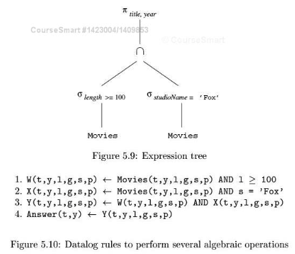
Converting Relational Algebra into Datalog

Datalog and Relational Algebra

  • A single, safe Datalog rule can be translated into Relational Algebra
  • That means that relational algebra and datalog can describe exactly the same queries
  • This class of queries is called relationally complete

  • But if you consider more than one datalog rule, things change
  • In particular, recursive datalog queries cannot be translated into relational algebra

  • Also, extended relational algebra cannot be translated into Datalog, but it can be translated into generalizations of Datalog, e.g., the Logic Data Language (LDL)

Datalog and GUIs

  • Query-by-Example (QBE) is an old database product that used a graphical query language
  • Microsoft Access is one of its famous descendants
  • Parts of QBE are also reinvented often by programmers writing web front-ends to database systems

  • QBE is very closely related to Datalog!

QBE Selection

QBE Selection

\[\sigma_{\text{rating=10}}(\text{Sailors})\]

QBE Join

QBE Join

\[\pi_{\text{sname}}((\text{Sailors} \bowtie \text{Reserves}) \bowtie_{\text{Reserves.bid=R2.bid}}(\rho_{\text{R2}}(\sigma_{\text{sid}=22}(\text{Reserves}))))\]

  • Notice how both joins and selections follow the same principles as Datalog